NAJZ Dev Research Lab · Biomechanics / Signal Modeling

The Jaggle Effect

Hamza LABBAALLI & Hassan OUAMMOU · University project · October 2026

Gluteal soft tissue after a heel strike behaves like a lightly damped mass–spring–damper. This page models it, applies Shannon information theory to the resulting signal, and lets you change the assumptions yourself. All parameters are assumptions pending measurement; this is an educational model, not a clinical conclusion.

Download full paper (PDF)Plain-text companion

3.8–5.8 Hznatural frequency, relaxed bodies

0.16–0.32damping ratio ζ (underdamped)

24–35 mmpeak displacement, running

0.25–0.65 stime to settle within 5 %

Interactive model

Move the sliders: the page recomputes f_n and ζ from the paper’s scaling laws and simulates a running heel-strike train (half-sine pulses, 0.06 s, 2.5 g).

Body mass M Body fat BF Shape factor σ Step frequency

relaxed muscle contracted compression garment

–natural frequency f_n

–damping ratio ζ

–resonance Q

–5 % settling time

–peak |z|

Dashed lines in the plot mark ±peak. The interactive uses a jitter-free periodic train, so peaks are about 12 % below the stochastic values in the tables.

1 · The model

Let z(t) be tissue displacement relative to the pelvis and a_b(t) the pelvis vertical acceleration:

z″ + 2ζωₙ z′ + ωₙ² z = −a_b(t) , ωₙ = √(k/m) , ζ = c / (2√(km))

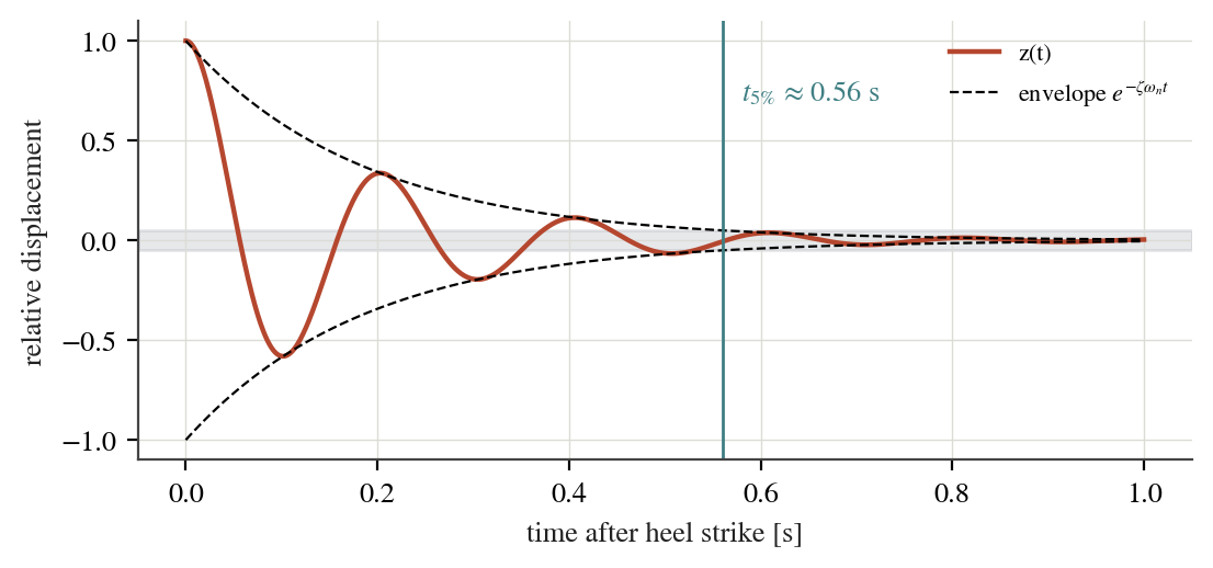
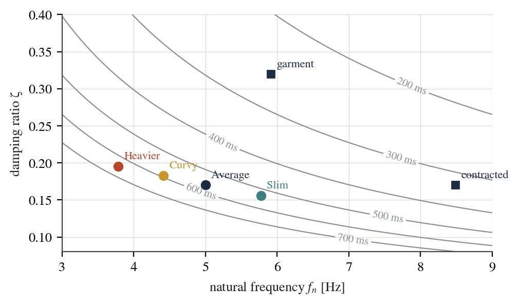
For ζ < 1 the tissue swings at ω_d = ω_n√(1−ζ²) and decays; that swinging is the jiggle. The decay is described by the logarithmic decrement and the 5 % settling time:

δ = ln(zₙ/zₙ₊₁) = 2πζ / √(1−ζ²) , t₅% ≈ 3 / (ζωₙ)

Dependence on body size, composition and shape

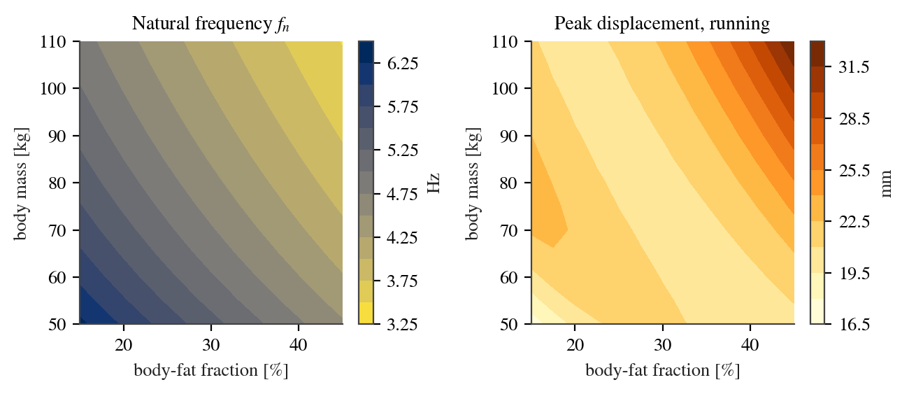
m_eff = M(0.02 + 0.06·BF) , E_eff = (1−BF)·Eₘ + BF·E_f , k = σ·C₀·E_eff·m_eff^(1/3)
fₙ = (1/2π)·√(σ C₀ E_eff / m_eff^(2/3)) ∝ m_eff^(−1/3) , ζ = (1−BF)·0.12 + BF·0.30

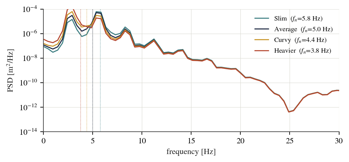
Heavier tissue lowers f_n (slower, larger jiggle), stiffer tissue raises it, and a wider, flatter shape (larger σ) raises it too. Calibration: the average relaxed body (65 kg, 28 % fat) has f_n = 5 Hz; muscle contraction multiplies E_m by 3, a garment multiplies k by 1.4 and sets ζ = 0.32.

Frequency response

|G| = 1 / (ωₙ²·√((1−r²)² + (2ζr)²)) , r = ω/ωₙ
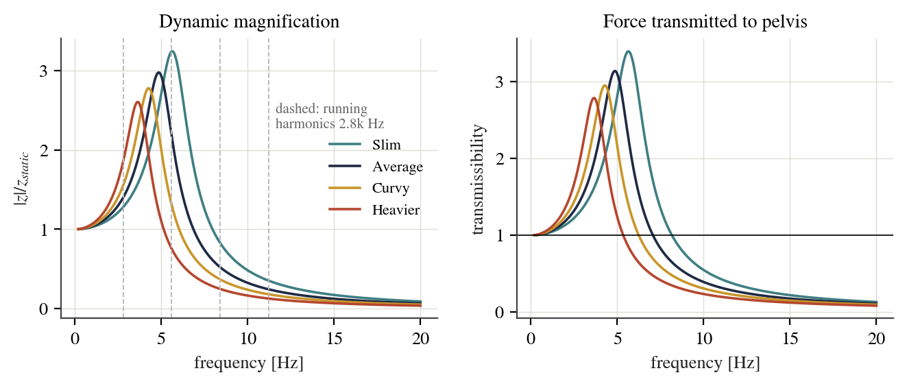
f_r = fₙ√(1−2ζ²) , Q ≈ 1/(2ζ) , Δf₋₃dB ≈ 2ζ fₙ , T(r) = √((1+(2ζr)²)/((1−r²)²+(2ζr)²))

Body	f_r Hz	Q	Δf Hz	δ	energy lost / cycle
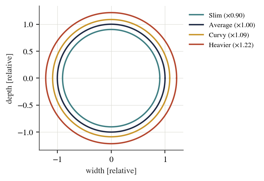
Slim	5.63	3.2	1.80	0.99	86 %
Average	4.85	3.0	1.70	1.09	89 %
Curvy	4.27	2.8	1.62	1.17	90 %
Heavier	3.64	2.6	1.48	1.25	92 %

Per cycle the vibration energy falls by e^−2δ, so the average body dissipates about 89 % of it every swing, which is why soft tissue matters for impact attenuation.

Dynamic magnification (left) and transmissibility (right). Dashed lines in the paper mark the running harmonics 2.8 k Hz.

The free response of the average case: a damped oscillation that settles in about half a second.

2 · Shannon information theory

H(Z) = −Σ pᵢ log₂ pᵢ [bit/sample] (displacement quantised at Δ = 0.25 mm)
Hₛ = −(1/log₂N) Σ P̂ₖ log₂ P̂ₖ ∈ [0,1] (spectral entropy, Welch PSD)
fₛ ≥ 2f_max (Nyquist) , C = B·log₂(1 + S/N) (Shannon–Hartley)

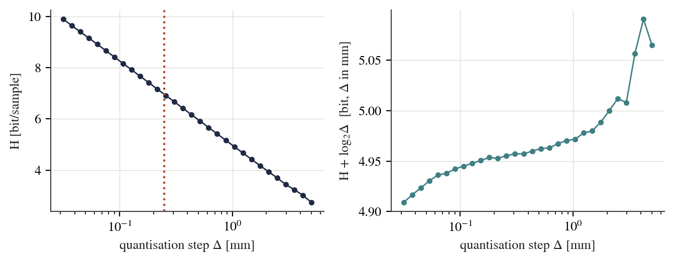
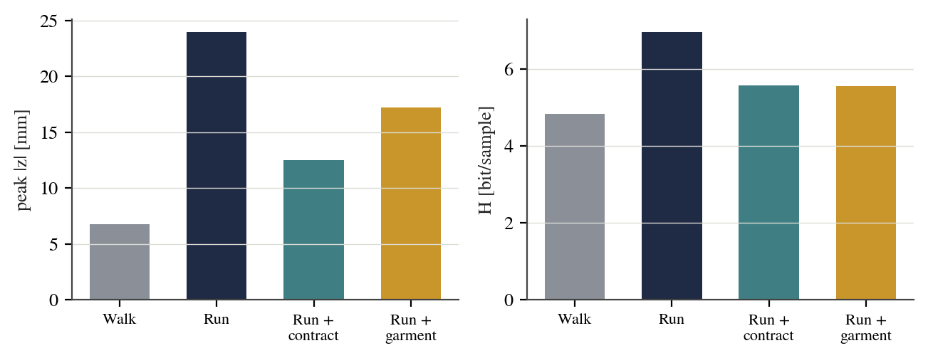
Entropy depends on the sensor. For small Δ, H ≈ h(Z) − log₂Δ: halving the step adds one bit. On the simulated signal H + log₂Δ stays flat at about 4.9 bit (Δ in mm) until Δ becomes coarse.

Sample entropy against quantisation step (left) and the invariant H + log₂Δ (right).

Worked sensor budget. 200 Hz sampling, ±40 mm range, Δ = 0.25 mm → 320 levels → 9-bit ADC. Running has H ≈ 6.96 bit, so a naive 1.39 kbit/s. A 50 Hz channel at 30 dB SNR has capacity ≈ 498 bit/s. The naive number is larger because neighbouring samples of an oscillation are correlated: sample entropy describes the signal but is not its bit rate.

Spectral entropy separates character from size: it is lowest for the heaviest body (0.32, energy concentrated at one resonance) and highest for the stiffened tissue (0.51).

3 · Results

Body size and composition (running, relaxed, σ = 1)

Type	M kg	BF %	m_eff kg	f_n Hz	ζ	Peak mm	RMS mm	t_5% ms	H bit	H_s
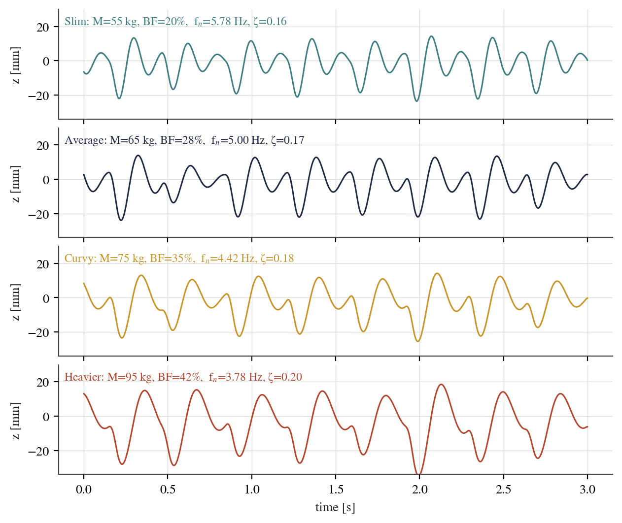
Slim	55	20	1.76	5.78	0.16	23.6	8.7	529	6.87	0.37
Average	65	28	2.39	5.00	0.17	24.0	8.9	560	6.96	0.41
Curvy	75	35	3.07	4.42	0.18	25.5	9.3	590	6.95	0.41
Heavier	95	42	4.29	3.78	0.20	34.7	12.6	645	7.37	0.32

Simulated tissue displacement for the four body types (3 s excerpt).

Natural frequency and peak running displacement over body mass and body fat.

Power spectral density; dotted lines mark each natural frequency.

Activity, muscle contraction and compression garment (65 kg, 28 % BF)

Condition	f_n Hz	ζ	Peak mm	RMS mm	t_5% ms	H bit	H_s
Walking, relaxed	5.00	0.17	6.8	2.2	560	4.83	0.47
Running, relaxed	5.00	0.17	24.0	8.9	560	6.96	0.41
Running, muscle contracted	8.49	0.17	12.5	3.8	330	5.57	0.51
Running, compression garment	5.91	0.32	17.2	5.1	252	5.56	0.45

Peak displacement and entropy by condition.

Tissue shape

Shape	σ	f_n Hz	Peak mm	RMS mm	H bit	H_s
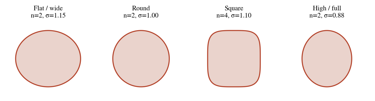
Flat / wide	1.15	5.36	23.7	8.9	6.90	0.38
Round	1.00	5.00	24.0	8.9	6.96	0.41
Square	1.10	5.24	24.0	8.9	6.92	0.39
High / full	0.88	4.69	24.5	9.0	6.97	0.42

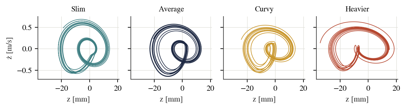
Design chart: settling-time contours on the natural-frequency / damping plane.

Phase portraits (displacement vs velocity) for the four bodies.

4 · Gait resonance

Amplitude depends on cadence as well as body. A running heel-strike train has energy at the step frequency and its harmonics; the jiggle peaks when a harmonic meets the tissue resonance. In the sweep the amplitude maxima fall at 2.87 steps/s (slim), 2.46 (average) and 2.17 (curvy), each close to f_n/2, the second harmonic.

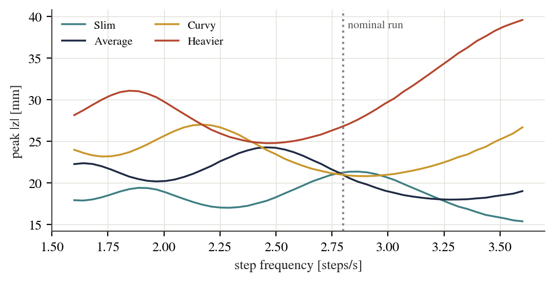
Peak displacement against step frequency.

So “heavier means bigger jiggle” is a tendency, not a law: shifting cadence away from a resonance reduces the motion.

5 · Sensitivity to the assumptions

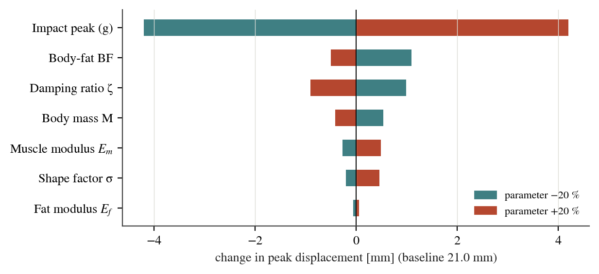
Each parameter was varied ±20 % around the average running case. Impact size dominates trivially (the model is linear); among tissue properties damping ratio and body fat matter most (≈ ±1 mm), then mass, muscle modulus and shape (≈ ±0.2–0.5 mm). Damping is therefore the first quantity worth measuring.

One-at-a-time sensitivity of peak displacement.

6 · A simulated population

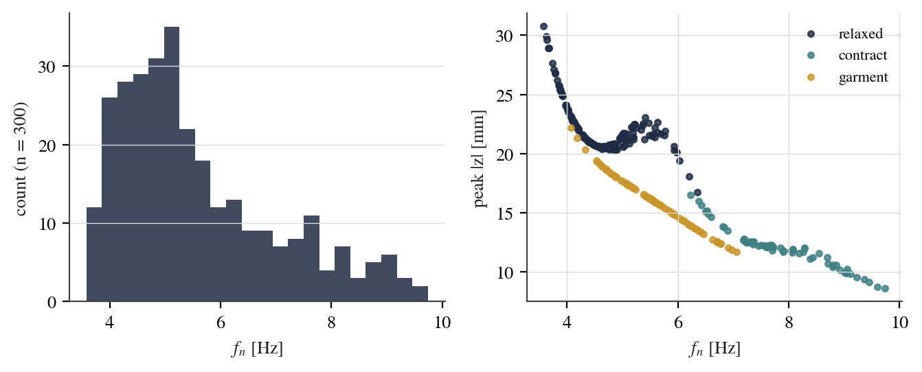
300 virtual bodies (50–110 kg, 15–45 % fat, varying shape, 25 % contracted and 25 % garment). Natural frequency averages 5.6 Hz (5–95 %: 3.9–8.7 Hz); peak displacement averages 18 mm (11–25 mm). Among relaxed bodies, peak ∝ f_n^−0.5 (correlation -0.68), while the correlation with body mass is only 0.46: frequency predicts amplitude better than mass does.

7 · Could it be measured?

Simulated test: fit the transfer function between pelvis and tissue acceleration from noisy 60 s records. The natural frequency is recovered to within about 2 % even at 5 dB SNR; damping is biased high by roughly 14–17 % (spectral resolution and leakage from the harmonic input), so it needs longer records or a time-domain fit to isolated decays.

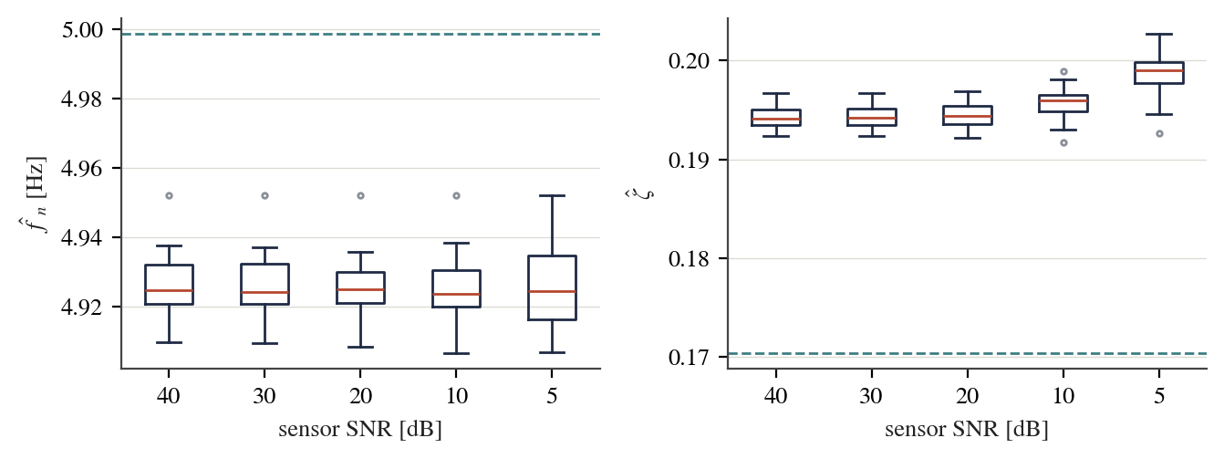
Recovered f<sub>n</sub> and ζ against sensor SNR (dashed = true value). — Recovered f_n and ζ against sensor SNR (dashed = true value).

Protocol: two IMUs (≥ 200 Hz), one on the sacrum and one on the gluteal belly, treadmill walking and running, relaxed / contracted / garment, at least 10 participants per predictor, informed consent and ethics approval.

8 · Geometry of the shape factor

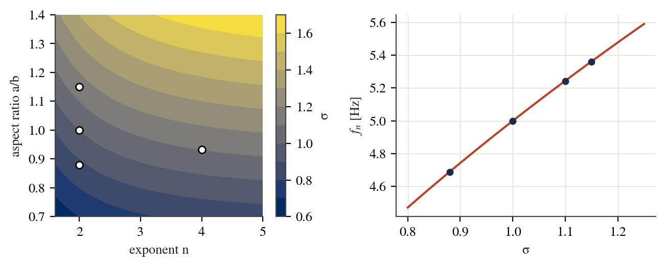
Tissue is drawn as a superellipse |x/a|ⁿ + |y/b|ⁿ = 1. The shape factor is σ = (a/b)·g(n)/g(2) with g(n) = Γ(1+1/n)² / Γ(1+2/n), so wide shallow tissue is stiffer and faster, tall deep tissue softer and slower. Since f_n ∝ √σ, a 15 % change in σ moves f_n by only about 7 %.

Superellipse cross-sections for the four shape classes.

Geometric similarity: outlines scaled by (m_eff / 2.39 kg)^(1/3).

σ over exponent n and aspect ratio a/b; f<sub>n</sub> against σ. — σ over exponent n and aspect ratio a/b; f_n against σ.

Limits

The model is one-dimensional and linear; moduli, damping ratios, C₀ and σ are assumed rather than measured; asymmetry and pelvic motion in other axes are ignored. Treat the numbers as trends. The next step is to measure real participants (with consent and ethics approval) and check whether real f_n and ζ match.